Hadoop basics

Server Roles in Hadoop

The three major categories of machine roles in a Hadoop deployment are Client machines, Masters nodes, and Slave nodes.  The Master nodes oversee the two key functional pieces that make up Hadoop: storing lots of data (HDFS), and running parallel computations on all that data (Map Reduce).  The Name Node oversees and coordinates the data storage function (HDFS), while the Job Tracker oversees and coordinates the parallel processing of data using Map Reduce.  Slave Nodes make up the vast majority of machines and do all the dirty work of storing the data and running the computations.  Each slave runs both a Data Node and Task Tracker daemon that communicate with and receive instructions from their master nodes.  The Task Tracker daemon is a slave to the Job Tracker, the Data Node daemon a slave to the Name Node.
Client machines have Hadoop installed with all the cluster settings, but are neither a Master or a Slave.  Instead, the role of the Client machine is to load data into the cluster, submit Map Reduce jobs describing how that data should be processed, and then retrieve or view the results of the job when its finished.  In smaller clusters (~40 nodes) you may have a single physical server playing multiple roles, such as both Job Tracker and Name Node.  With medium to large clusters you will often have each role operating on a single server machine.
In real production clusters there is no server virtualization, no hypervisor layer.  That would only amount to unnecessary overhead impeding performance.  Hadoop runs best on Linux machines, working directly with the underlying hardware.  That said, Hadoop does work in a virtual machine.  That’s a great way to learn and get Hadoop up and running fast and cheap.  I have a 6-node cluster up and running in VMware Workstation on my Windows 7 laptop.

---

Hadoop Cluster

This is the typical architecture of a Hadoop cluster.  You will have rack servers (not blades) populated in racks connected to a top of rack switch usually with 1 or 2 GE boned links.  10GE nodes are uncommon but gaining interest as machines continue to get more dense with CPU cores and disk drives.  The rack switch has uplinks connected to another tier of switches connecting all the other racks with uniform bandwidth, forming the cluster.  The majority of the servers will be Slave nodes with lots of local disk storage and moderate amounts of CPU and DRAM.  Some of the machines will be Master nodes that might have a slightly different configuration favoring more DRAM and CPU, less local storage.
In this post, we are not going to discuss various detailed network design options.  Let’s save that for another discussion (stay tuned).  First, lets understand how this application works…

---

Hadoop Workflow

Why did Hadoop come to exist? What problem does it solve?  Simply put, businesses and governments have a tremendous amount of data that needs to be analyzed and processed very quickly.  If I can chop that huge chunk of data into small chunks and spread it out over many machines, and have all those machines processes their portion of the data in parallel — I can get answers extremely fast — and that, in a nutshell, is what Hadoop does.
In our simple example, we’ll have a huge data file containing emails sent to the customer service department.  I want a quick snapshot to see how many times the word “Refund” was typed by my customers.  This might help me to anticipate the demand on our returns and exchanges department, and staff it appropriately.  It’s a simple word count exercise.  The Client will load the data into the cluster (File.txt), submit a job describing how to analyze that data (word count), the cluster will store the results in a new file (Results.txt), and the Client will read the results file.

---

Writing Files to HDFS

Your Hadoop cluster is useless until it has data, so we’ll begin by loading our huge File.txt into the cluster for processing.  The goal here is fast parallel processing of lots of data.  To accomplish that I need as many machines as possible working on this data all at once.  To that end, the Client is going to break the data file into smaller “Blocks”, and place those blocks on different machines throughout the cluster.  The more blocks I have, the more machines that will be able to work on this data in parallel.  At the same time, these machines may be prone to failure, so I want to insure that every block of data is on multiple machines at once to avoid data loss.  So each block will be replicated in the cluster as its loaded.  The standard setting for Hadoop is to have (3) copies of each block in the cluster.  This can be configured with the dfs.replication parameter in the file hdfs-site.xml.
The Client breaks File.txt into (3) Blocks.  For each block, the Client consults the Name Node (usually TCP 9000) and receives a list of (3) Data Nodes that should have a copy of this block.  The Client then writes the block directly to the Data Node (usually TCP 50010).  The receiving Data Node replicates the block to other Data Nodes, and the cycle repeats for the remaining blocks.  The Name Node is not in the data path.  The Name Node only provides the map of where data is and where data should go in the cluster (file system metadata).

---

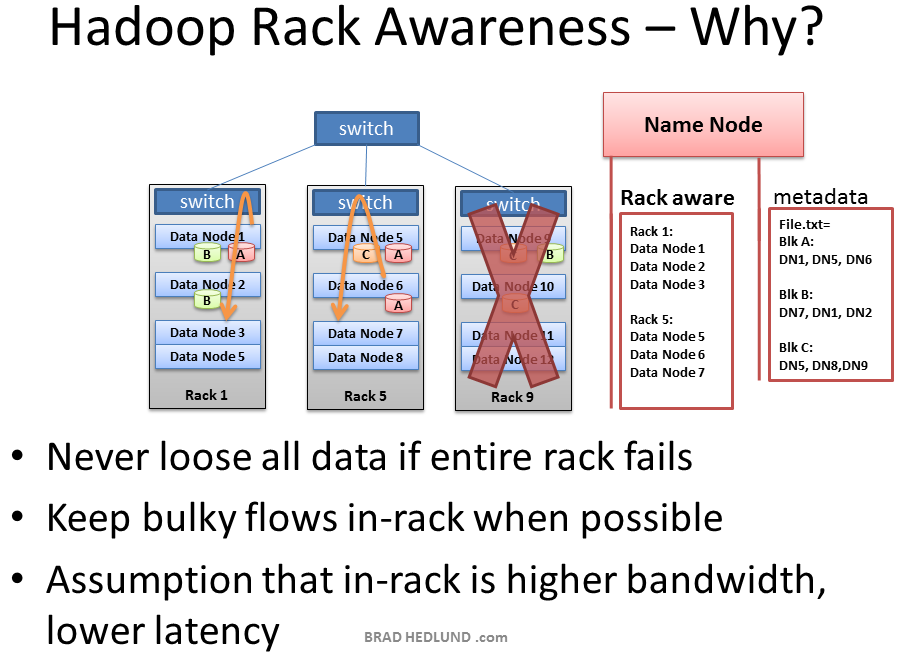
Hadoop Rack Awareness

Hadoop has the concept of “Rack Awareness”.  As the Hadoop administrator you can manually define the rack number of each slave Data Node in your cluster.  Why would you go through the trouble of doing this?  There are two key reasons for this: Data loss prevention, and network performance.  Remember that each block of data will be replicated to multiple machines to prevent the failure of one machine from losing all copies of data.  Wouldn’t it be unfortunate if all copies of data happened to be located on machines in the same rack, and that rack experiences a failure? Such as a switch failure or power failure.  That would be a mess.  So to avoid this, somebody needs to know where Data Nodes are located in the network topology and use that information to make an intelligent decision about where data replicas should exist in the cluster.  That “somebody” is the Name Node.
There is also an assumption that two machines in the same rack have more bandwidth and lower latency between each other than two machines in two different racks.  This is true most of the time.  The rack switch uplink bandwidth is usually (but not always) less than its downlink bandwidth.  Furthermore, in-rack latency is usually lower than cross-rack latency (but not always).  If at least one of those two basic assumptions are true, wouldn’t it be cool if Hadoop can use the same Rack Awareness that protects data to also optimally place work streams in the cluster, improving network performance?  Well, it does! Cool, right?
What is NOT cool about Rack Awareness at this point is the manual work required to define it the first time, continually update it, and keep the information accurate.  If the rack switch could auto-magically provide the Name Node with the list of Data Nodes it has, that would be cool. Or vice versa, if the Data Nodes could auto-magically tell the Name Node what switch they’re connected to, that would be cool too.
Even more interesting would be a OpenFlow network, where the Name Node could query the OpenFlow controller about a Node’s location in the topology.

---

Preparing HDFS Writes

The Client is ready to load File.txt into the cluster and breaks it up into blocks, starting with Block A.  The Client consults the Name Node that it wants to write File.txt, gets permission from the Name Node, and receives a list of (3) Data Nodes for each block, a unique list for each block.  The Name Node used its Rack Awareness data to influence the decision of which Data Nodes to provide in these lists.  The key rule is that for every block of data, two copies will exist in one rack, another copy in a different rack.  So the list provided to the Client will follow this rule.
Before the Client writes “Block A” of File.txt to the cluster it wants to know that all Data Nodes which are expected to have a copy of this block are ready to receive it.  It picks the first Data Node in the list for Block A (Data Node 1), opens a TCP 50010 connection and says, “Hey, get ready to receive a block, and here’s a list of (2) Data Nodes, Data Node 5 and Data Node 6.  Go make sure they’re ready to receive this block too.”  Data Node 1 then opens a TCP connection to Data Node 5 and says, “Hey, get ready to receive a block, and go make sure Data Node 6 is ready is receive this block too.”  Data Node 5 will then ask Data Node 6, “Hey, are you ready to receive a block?”
The acknowledgments of readiness come back on the same TCP pipeline, until the initial Data Node 1 sends a “Ready” message back to the Client.  At this point the Client is ready to begin writing block data into the cluster.

---

HDFS Write Pipeline

As data for each block is written into the cluster a replication pipeline is created between the (3) Data Nodes (or however many you have configured in dfs.replication).  This means that as a Data Node is receiving block data it will at the same time push a copy of that data to the next Node in the pipeline.
Here too is a primary example of leveraging the Rack Awareness data in the Name Node to improve cluster performance.  Notice that the second and third Data Nodes in the pipeline are in the same rack, and therefore the final leg of the pipeline does not need to traverse between racks and instead benefits from in-rack bandwidth and low latency.  The next block will not be begin until this block is successfully written to all three nodes.

---

HDFS Pipeline Write Success

When all three Nodes have successfully received the block they will send a “Block Received” report to the Name Node.  They will also send “Success” messages back up the pipeline and close down the TCP sessions.  The Client receives a success message and tells the Name Node the block was successfully written.  The Name Node updates it metadata info with the Node locations of Block A in File.txt.
The Client is ready to start the pipeline process again for the next block of data.

---

HDFS Multi-block Replication Pipeline

As the subsequent blocks of File.txt are written, the initial node in the pipeline will vary for each block, spreading around the hot spots of in-rack and cross-rack traffic for replication.
Hadoop uses a lot of network bandwidth and storage.  We are typically dealing with very big files, Terabytes in size.  And each file will be replicated onto the network and disk (3) times.  If you have a 1TB file it will consume 3TB of network traffic to successfully load the file, and 3TB disk space to hold the file.

---

Client Writes Span Cluster

After the replication pipeline of each block is complete the file is successfully written to the cluster.  As intended the file is spread in blocks across the cluster of machines, each machine having a relatively small part of the data.  The more blocks that make up a file, the more machines the data can potentially spread.  The more CPU cores and disk drives that have a piece of my data mean more parallel processing power and faster results.  This is the motivation behind building large, wide clusters.  To process more data, faster.  When the machine count goes up and the cluster goes wide, our network needs to scale appropriately.
Another approach to scaling the cluster is to go deep. This is where you scale up the machines with more disk drives and more CPU cores.  Instead of increasing the number of machines you begin to look at increasing the density of each machine.  In scaling deep, you put yourself on a trajectory where more network I/O requirements may be demanded of fewer machines.  In this model, how your Hadoop cluster makes the transition to 10GE nodes becomes an important consideration.

---

Name Node

The Name Node holds all the file system metadata for the cluster and oversees the health of Data Nodes and coordinates access to data.  The Name Node is the central controller of HDFS.  It does not hold any cluster data itself.  The Name Node only knows what blocks make up a file and where those blocks are located in the cluster.  The Name Node points Clients to the Data Nodes they need to talk to and keeps track of the cluster’s storage capacity, the health of each Data Node, and making sure each block of data is meeting the minimum defined replica policy.
Data Nodes send heartbeats to the Name Node every 3 seconds via a TCP handshake, using the same port number defined for the Name Node daemon, usually TCP 9000.  Every tenth heartbeat is a Block Report, where the Data Node tells the Name Node about all the blocks it has.  The block reports allow the Name Node build its metadata and insure (3) copies of the block exist on different nodes, in different racks.
The Name Node is a critical component of the Hadoop Distributed File System (HDFS).  Without it, Clients would not be able to write or read files from HDFS, and it would be impossible to schedule and execute Map Reduce jobs.  Because of this, it’s a good idea to equip the Name Node with a highly redundant enterprise class server configuration; dual power supplies, hot swappable fans, redundant NIC connections, etc.

---

Re-replicating Missing Replicas

If the Name Node stops receiving heartbeats from a Data Node it presumes it to be dead and any data it had to be gone as well.  Based on the block reports it had been receiving from the dead node, the Name Node knows which copies of blocks died along with the node and can make the decision to re-replicate those blocks to other Data Nodes.  It will also consult the Rack Awareness data in order to maintain the two copies in one rack, one copy in another rack replica rule when deciding which Data Node should receive a new copy of the blocks.
Consider the scenario where an entire rack of servers falls off the network, perhaps because of a rack switch failure, or power failure.  The Name Node would begin instructing the remaining nodes in the cluster to re-replicate all of the data blocks lost in that rack.  If each server in that rack had a modest 12TB of data, this could be hundreds of terabytes of data that needs to begin traversing the network.

---

Secondary Name Node

Hadoop has server role called the Secondary Name Node.  A common misconception is that this role provides a high availability backup for the Name Node.  This is not the case.
The Secondary Name Node occasionally connects to the Name Node (by default, ever hour) and grabs a copy of the Name Node’s in-memory metadata and files used to store metadata (both of which may be out of sync).  The Secondary Name Node combines this information in a fresh set of files and delivers them back to the Name Node, while keeping a copy for itself.
Should the Name Node die, the files retained by the Secondary Name Node can be used to recover the Name Node.  In a busy cluster, the administrator may configure the Secondary Name Node to provide this housekeeping service much more frequently than the default setting of one hour.  Maybe every minute.

---

Client Read from HDFS

When a Client wants to retrieve a file from HDFS, perhaps the output of a job, it again consults the Name Node and asks for the block locations of the file.  The Name Node returns a list of each Data Node holding a block, for each block.
The Client picks a Data Node from each block list and reads one block at a time with TCP on port 50010, the default port number for the Data Node daemon.  It does not progress to the next block until the previous block completes.

---

Data Node reads from HDFS

There are some cases in which a Data Node daemon itself will need to read a block of data from HDFS.  One such case is where the Data Node has been asked to process data that it does not have locally, and therefore it must retrieve the data from another Data Node over the network before it can begin processing.
This is another key example of the Name Node’s Rack Awareness knowledge providing optimal network behavior.  When the Data Node asks the Name Node for location of block data, the Name Node will check if another Data Node in the same rack has the data.  If so, the Name Node provides the in-rack location from which to retrieve the data.  The flow does not need to traverse two more switches and congested links find the data in another rack.  With the data retrieved quicker in-rack, the data processing can begin sooner, and the job completes that much faster.

---

Map Task

Now that File.txt is spread in small blocks across my cluster of machines I have the opportunity to provide extremely fast and efficient parallel processing of that data.  The parallel processing framework included with Hadoop is called Map Reduce, named after two important steps in the model; Map, and Reduce.
The first step is the Map process.  This is where we simultaneously ask our machines to run a computation on their local block of data.  In this case we are asking our machines to count the number of occurrences of the word “Refund” in the data blocks of File.txt.
To start this process the Client machine submits the Map Reduce job to the Job Tracker, asking “How many times does Refund occur in File.txt” (paraphrasing Java code).  The Job Tracker consults the Name Node to learn which Data Nodes have blocks of File.txt.  The Job Tracker then provides the Task Tracker running on those nodes with the Java code required to execute the Map computation on their local data.  The Task Tracker starts a Map task and monitors the tasks progress.  The Task Tracker provides heartbeats and task status back to the Job Tracker.
As each Map task completes, each node stores the result of its local computation in temporary local storage.  This is called the “intermediate data”.  The next step will be to send this intermediate data over the network to a Node running a Reduce task for final computation.

---

What if Map Task data isn’t local?

While the Job Tracker will always try to pick nodes with local data for a Map task, it may not always be able to do so.  One reason for this might be that all of the nodes with local data already have too many other tasks running and cannot accept anymore.
In this case, the Job Tracker will consult the Name Node whose Rack Awareness knowledge can suggest other nodes in the same rack.  The Job Tracker will assign the task to a node in the same rack, and when that node goes to find the data it needs the Name Node will instruct it to grab the data from another node in its rack, leveraging the presumed single hop and high bandwidth of in-rack switching.

---

Reduce Task computes data received from Map Tasks

The second phase of the Map Reduce framework is called, you guess it, Reduce.  The Map task on the machines have completed and generated their intermediate data.  Now we need to gather all of this intermediate data to combine and distill it for further processing such that we have one final result.
The Job Tracker starts a Reduce task on any one of the nodes in the cluster and instructs the Reduce task to go grab the intermediate data from all of the completed Map tasks.  The Map tasks may respond to the Reducer almost simultaneously, resulting in a situation where you have a number of nodes sending TCP data to a single node, all at once.  This traffic condition is often referred to as “Incast” or “fan-in”.  For networks handling lots of incast conditions, its important the network switches have well-engineered internal traffic management capabilities, and adequate buffers (not too big, not too small).  Throwing gobs of buffers at a switch may end up causing unwanted collateral damage to other traffic.  But that’s a topic for another day.
The Reducer task has now collected all of the intermediate data from the Map tasks and can begin the final computation phase.  In this case, we are simply adding up the sum total occurrences of the word “Refund” and writing the result to a file called Results.txt
The output from the job is a file called Results.txt that is written to HDFS following all of the processes we have covered already; splitting the file up into blocks, pipeline replication of those blocks, etc.  When complete, the Client machine can read the Results.txt file from HDFS, and the job is considered complete.
Our simple word count job did not result in a lot of intermediate data to transfer over the network.  Other jobs however may produce a lot of intermediate data — such as sorting a terabyte of data.  Where the output of the Map Reduce job is a new set of data equal to the size of data you started with.  How much traffic you see on the network in the Map Reduce process is entirely dependent on the type job you are running at that given time.
If you’re a studious network administrator, you would learn more about Map Reduce and the types of jobs your cluster will be running, and how the type of job affects the traffic flows on your network.  If you’re a Hadoop networking rock star, you might even be able to suggest ways to better code the Map Reduce jobs so as to optimize the performance of the network, resulting in faster job completion times.

---

Unbalanced Hadoop Cluster

Hadoop may start to be a real success in your organization, providing a lot of previously untapped business value from all that data sitting around.  When business folks find out about this you can bet that you’ll quickly have more money to buy more racks of servers and network for your Hadoop cluster.
When you add new racks full of servers and network to an existing Hadoop cluster you can end up in a situation where your cluster is unbalanced.  In this case, Racks 1 & 2 were my existing racks containing File.txt and running my Map Reduce jobs on that data.  When I added two new racks to the cluster, my File.txt data doesn’t auto-magically start spreading over to the new racks.  All the data stays where it is.
The new servers are sitting idle with no data, until I start loading new data into the cluster.  Furthermore, if the servers in Racks 1 & 2 are really busy, the Job Tracker may have no other choice but to assign Map tasks on File.txt to the new servers which have no local data.  The new servers need to go grab the data over the network.  As as result you may see more network traffic and slower job completion times.

---

Hadoop Cluster Balancer

To fix the unbalanced cluster situation, Hadoop includes a nifty utility called, you guessed it, balancer.
Balancer looks at the difference in available storage between nodes and attempts to provide balance to a certain threshold.  New nodes with lots of free disk space will be detected and balancer can begin copying block data off nodes with less available space to the new nodes.  Balancer isn’t running until someone types the command at a terminal, and it stops when the terminal is canceled or closed.
The amount of network traffic balancer can use is very low, with a default setting of 1MB/s.  This setting can be changed with the dfs.balance.bandwidthPerSec parameter in the file hdfs-site.xml
The Balancer is good housekeeping for your cluster.  It should definitely be used any time new machines are added, and perhaps even run once a week for good measure.  Given the balancers low default bandwidth setting it can take a long time to finish its work, perhaps days or weeks.

Resource:http://bradhedlund.com/2011/09/10/understanding-hadoop-clusters-and-the-network/

Exploring the software behind Facebook, the world’s largest site

77
inShare

At the scale that Facebook operates, a lot of traditional approaches to serving web content break down or simply aren’t practical. The challenge for Facebook’s engineers has been to keep the site up and running smoothly in spite of handling close to half a billion active users. This article takes a look at some of the software and techniques they use to accomplish that.

Facebook’s scaling challenge

Before we get into the details, here are a few factoids to give you an idea of the scaling challenge that Facebook has to deal with:

• Facebook serves 570 billion page views per month (according to Google Ad Planner).
• There are more photos on Facebook than all other photo sites combined (including sites like Flickr).
• More than 3 billion photos are uploaded every month.
• Facebook’s systems serve 1.2 million photos per second. This doesn’t include the images served by Facebook’s CDN.
• More than 25 billion pieces of content (status updates, comments, etc) are shared every month.
• Facebook has more than 30,000 servers (and this number is from last year!)

Software that helps Facebook scale

In some ways Facebook is still a LAMP site (kind of), but it has had to change and extend its operation to incorporate a lot of other elements and services, and modify the approach to existing ones.
For example:

• Facebook still uses PHP, but it has built a compiler for it so it can be turned into native code on its web servers, thus boosting performance.
• Facebook uses Linux, but has optimized it for its own purposes (especially in terms of network throughput).
• Facebook uses MySQL, but primarily as a key-value persistent storage, moving joins and logic onto the web servers since optimizations are easier to perform there (on the “other side” of the Memcached layer).

Then there are the custom-written systems, like Haystack, a highly scalable object store used to serve Facebook’s immense amount of photos, or Scribe, a logging system that can operate at the scale of Facebook (which is far from trivial).
But enough of that. Let’s present (some of) the software that Facebook uses to provide us all with the world’s largest social network site.

Memcached

Memcached is by now one of the most famous pieces of software on the internet. It’s a distributed memory caching system which Facebook (and a ton of other sites) use as a caching layer between the web servers and MySQL servers (since database access is relatively slow). Through the years, Facebook has made a ton of optimizations to Memcached and the surrounding software (like optimizing the network stack).
Facebook runs thousands of Memcached servers with tens of terabytes of cached data at any one point in time. It is likely the world’s largest Memcached installation.

HipHop for PHP

PHP, being a scripting language, is relatively slow when compared to code that runs natively on a server. HipHop converts PHP into C++ code which can then be compiled for better performance. This has allowed Facebook to get much more out of its web servers since Facebook relies heavily on PHP to serve content.
A small team of engineers (initially just three of them) at Facebook spent 18 months developing HipHop, and it is now live in production.

Haystack

Haystack is Facebook’s high-performance photo storage/retrieval system (strictly speaking, Haystack is an object store, so it doesn’t necessarily have to store photos). It has a ton of work to do; there are more than 20 billion uploaded photos on Facebook, and each one is saved in four different resolutions, resulting in more than 80 billion photos.
And it’s not just about being able to handle billions of photos, performance is critical. As we mentioned previously, Facebook serves around 1.2 million photos per second, a number which doesn’t include images served by Facebook’s CDN. That’s a staggering number.

BigPipe

BigPipe is a dynamic web page serving system that Facebook has developed. Facebook uses it to serve each web page in sections (called “pagelets”) for optimal performance.
For example, the chat window is retrieved separately, the news feed is retrieved separately, and so on. These pagelets can be retrieved in parallel, which is where the performance gain comes in, and it also gives users a site that works even if some part of it would be deactivated or broken.

Cassandra

Cassandra is a distributed storage system with no single point of failure. It’s one of the poster children for the NoSQL movement and has been made open source (it’s even become an Apache project). Facebook uses it for its Inbox search.
Other than Facebook, a number of other services use it, for example Digg. We’re even considering some uses for it here at Pingdom.

Scribe

Scribe is a flexible logging system that Facebook uses for a multitude of purposes internally. It’s been built to be able to handle logging at the scale of Facebook, and automatically handles new logging categories as they show up (Facebook has hundreds).

Hadoop and Hive

Hadoop is an open source map-reduce implementation that makes it possible to perform calculations on massive amounts of data. Facebook uses this for data analysis (and as we all know, Facebook has massive amounts of data). Hive originated from within Facebook, and makes it possible to use SQL queries against Hadoop, making it easier for non-programmers to use.
Both Hadoop and Hive are open source (Apache projects) and are used by a number of big services, for example Yahoo and Twitter.

Thrift

Facebook uses several different languages for its different services. PHP is used for the front-end, Erlang is used for Chat, Java and C++ are also used in several places (and perhaps other languages as well). Thrift is an internally developed cross-language framework that ties all of these different languages together, making it possible for them to talk to each other. This has made it much easier for Facebook to keep up its cross-language development.
Facebook has made Thrift open source and support for even more languages has been added.

Varnish

Varnish is an HTTP accelerator which can act as a load balancer and also cache content which can then be served lightning-fast.
Facebook uses Varnish to serve photos and profile pictures, handling billions of requests every day. Like almost everything Facebook uses, Varnish is open source.

Other things that help Facebook run smoothly

We have mentioned some of the software that makes up Facebook’s system(s) and helps the service scale properly. But handling such a large system is a complex task, so we thought we would list a few more things that Facebook does to keep its service running smoothly.

Gradual releases and dark launches

Facebook has a system they called Gatekeeper that lets them run different code for different sets of users (it basically introduces different conditions in the code base). This lets Facebook do gradual releases of new features, A/B testing, activate certain features only for Facebook employees, etc.
Gatekeeper also lets Facebook do something called “dark launches”, which is to activate elements of a certain feature behind the scenes before it goes live (without users noticing since there will be no corresponding UI elements). This acts as a real-world stress test and helps expose bottlenecks and other problem areas before a feature is officially launched. Dark launches are usually done two weeks before the actual launch.

Profiling of the live system

Facebook carefully monitors its systems (something we here at Pingdom of course approve of), and interestingly enough it also monitors the performance of every single PHP function in the live production environment. This profiling of the live PHP environment is done using an open source tool called XHProf.

Gradual feature disabling for added performance

If Facebook runs into performance issues, there are a large number of levers that let them gradually disable less important features to boost performance of Facebook’s core features.

The things we didn’t mention

We didn’t go much into the hardware side in this article, but of course that is also an important aspect when it comes to scalability. For example, like many other big sites, Facebook uses a CDN to help serve static content. And then of course there is the huge data center Facebook is building in Oregon to help it scale out with even more servers.
And aside from what we have already mentioned, there is of course a ton of other software involved. However, we hope we were able to highlight some of the more interesting choices Facebook has made.

Facebook’s love affair with open source

We can’t complete this article without mentioning how much Facebook likes open source. Or perhaps we should say, “loves”.
Not only is Facebook using (and contributing to) open source software such as Linux, Memcached, MySQL, Hadoop, and many others, it has also made much of its internally developed software available as open source.
Examples of open source projects that originated from inside Facebook include HipHop, Cassandra, Thrift and Scribe. Facebook has also open-sourced Tornado, a high-performance web server framework developed by the team behind FriendFeed (which Facebook bought in August 2009).
(A list of open source software that Facebook is involved with can be found on Facebook’s Open Source page.)

More scaling challenges to come

Facebook has been growing at an incredible pace. Its user base is increasing almost exponentially and is now close to half a billion active users, and who knows what it will be by the end of the year. The site seems to be growing with about 100 million users every six months or so.
Facebook even has a dedicated “growth team” that constantly tries to figure out how to make people use and interact with the site even more.
This rapid growth means that Facebook will keep running into various performance bottlenecks as it’s challenged by more and more page views, searches, uploaded images, status messages, and all the other ways that Facebook users interact with the site and each other.
But this is just a fact of life for a service like Facebook. Facebook’s engineers will keep iterating and coming up with new ways to scale (it’s not just about adding more servers). For example, Facebook’s photo storage system has already been completely rewritten several times as the site has grown.
So, we’ll see what the engineers at Facebook come up with next. We bet it’s something interesting. After all, they are scaling a mountain that most of us can only dream of; a site with more users than most countries. When you do that, you better get creative.

Resource:http://royal.pingdom.com/2010/06/18/the-software-behind-facebook/

Hive tutorial

CREATE TABLE creates a table with the given name. An error is thrown if a table or view with the same name already exists. Use IF NOT EXISTS to skip the error.
The EXTERNAL keyword lets you create a table and provide a LOCATION so that Hive does not use a default location for this table. This comes in handy if you already have data generated. When dropping an EXTERNAL table, data in the table is NOT deleted from the file system.
The LIKE form of CREATE TABLE allows you to copy an existing table definition exactly (without copying its data).
You can create tables with custom SerDe or using native SerDe. A native SerDe is used if ROW FORMAT is not specified or ROW FORMAT DELIMITED is specified. You can use the DELIMITED clause to read delimited files. Use the SERDE clause to create a table with custom SerDe. 
You must specify a list of a columns for tables that use a native SerDe. A list of columns for tables that use a custom SerDe may be specified but Hive will query the SerDe to determine the actual list of columns for this table.
Use STORED AS TEXTFILE if the data needs to be stored as plain text files. Use STORED AS SEQUENCEFILE if the data needs to be compressed. Please read more about Hive/CompressedStorage if you are planning to keep data compressed in your Hive tables. Use INPUTFORMAT and OUTPUTFORMAT to specify the name of a corresponding InputFormat and OutputFormat class as a string literal, e.g. 'org.apache.hadoop.hive.contrib.fileformat.base64.Base64TextInputFormat'.
Use STORED BY to create a non-native table, for example in HBase. See Hive/StorageHandlers for more information on this option.
Partitioned tables can be created using the PARTITIONED BY clause. A table can have one or more partition columns and a separate data directory is created for each distinct value combination in the partition columns. Further, tables or partitions can be bucketed using CLUSTERED BY columns, and data can be sorted within that bucket via SORT BY columns. This can be used to improve performance on certain kinds of queries.
Table names and column names are case insensitive but SerDe and property names are case sensitive. Table and column comments are string literals (single-quoted). The TBLPROPERTIES clause allows you to tag the table definition with your own metadata key/value pairs.
Tables can also be created and populated by the results of a query in one create-table-as-select (CTAS) statement. The table created by CTAS is atomic, meaning that the table is not seen by other users until all the query results are populated. So other users will either see the table with the complete results of the query or will not see the table at all.
There are two parts in CTAS, the SELECT part can be any SELECT statement supported by HiveQL. The CREATE part of the CTAS takes the resulting schema from the SELECT part and creates the target table with other table properties such as the SerDe and storage format. The only restrictions in CTAS is that the target table cannot be a partitioned table (nor can it be an external table).
Examples:
Here's an example statement to create a table:

CREATE TABLE page_view(viewTime INT, userid BIGINT,
     page_url STRING, referrer_url STRING,
     ip STRING COMMENT 'IP Address of the User')
 COMMENT 'This is the page view table'
 PARTITIONED BY(dt STRING, country STRING)
 STORED AS SEQUENCEFILE;

The statement above creates the page_view table with viewTime, userid, page_url, referrer_url, and ip columns (including comments). The table is also partitioned and data is stored in sequence files. The data format in the files is assumed to be field-delimited by ctrl-A and row-delimited by newline.

CREATE TABLE page_view(viewTime INT, userid BIGINT,
     page_url STRING, referrer_url STRING,
     ip STRING COMMENT 'IP Address of the User')
 COMMENT 'This is the page view table'
 PARTITIONED BY(dt STRING, country STRING)
 ROW FORMAT DELIMITED
   FIELDS TERMINATED BY '\001'
STORED AS SEQUENCEFILE;

The above statement lets you create the same table as the previous table.

CREATE TABLE page_view(viewTime INT, userid BIGINT,
     page_url STRING, referrer_url STRING,
     ip STRING COMMENT 'IP Address of the User')
 COMMENT 'This is the page view table'
 PARTITIONED BY(dt STRING, country STRING)
 CLUSTERED BY(userid) SORTED BY(viewTime) INTO 32 BUCKETS
 ROW FORMAT DELIMITED
   FIELDS TERMINATED BY '\001'
   COLLECTION ITEMS TERMINATED BY '\002'
   MAP KEYS TERMINATED BY '\003'
 STORED AS SEQUENCEFILE;

In the example above, the page_view table is bucketed (clustered by) userid and within each bucket the data is sorted in increasing order of viewTime. Such an organization allows the user to do efficient sampling on the clustered column - in this case userid. The sorting property allows internal operators to take advantage of the better-known data structure while evaluating queries, also increasing efficiency. MAP KEYS and COLLECTION ITEMS keywords can be used if any of the columns are lists or maps.
In all the examples until now the data is stored in the Hive Metadata Store in the sub-directory page_view.

CREATE EXTERNAL TABLE page_view(viewTime INT, userid BIGINT,
     page_url STRING, referrer_url STRING,
     ip STRING COMMENT 'IP Address of the User',
     country STRING COMMENT 'country of origination')
 COMMENT 'This is the staging page view table'
 ROW FORMAT DELIMITED FIELDS TERMINATED BY '\054'
 STORED AS TEXTFILE
 LOCATION '';

You can use the above statement to create a page_view table which points to any hdfs location for its storage. But you still have to make sure that the data is delimited as specified in the query above.

CREATE TABLE new_key_value_store
   ROW FORMAT SERDE "org.apache.hadoop.hive.serde2.columnar.ColumnarSerDe"
   STORED AS RCFile AS
SELECT (KEY % 1024) new_key, concat(KEY, value) key_value_pair
FROM key_value_store
SORT BY new_key, key_value_pair;

The above CTAS statement creates the target table new_key_value_store with the schema (new_key DOUBLE, key_value_pair STRING) derived from the results of the SELECT statement. If the SELECT statement does not specify column aliases, the column names will be automatically assigned to _col0, _col1, and _col2 etc. In addition, the new target table is created using a specific SerDe and a storage format independent of the source tables in the SELECT statement.
Before using this command, the table key_value_store can be created and loaded as follows:

CREATE TABLE key_value_store (
    KEY int,
    value string
)
    ROW FORMAT DELIMITED FIELDS TERMINATED BY '\t'
    STORED AS TEXTFILE;

LOAD DATA LOCAL INPATH 'file:///C:/Users/nkaushik/Desktop/key_value.txt'
INTO TABLE key_value_store;

The file key_value.txt is tab delimited and contains the following entries:

1    :value_1
2    :value_2
3    :value_3
4    :value_4
5    :value_5

CREATE TABLE empty_key_value_store
LIKE key_value_store;

In contrast, the statement above creates a new empty_key_value_store table whose definition exactly matches the existing key_value_store in all particulars other than table name. The new table contains no rows.

Inserting Data Into Bucketed Tables

The CLUSTERED BY and SORTED BY creation commands do not affect how data is inserted into a table -- only how it is read. This means that users must be careful to insert data correctly by specifying the number of reducers to be equal to the number of buckets, and using CLUSTER BY and SORT BY commands in their query.
There is also an example of creating and populating bucketed tables.

Drop Table

DROP TABLE table_name

DROP TABLE removes metadata and data for this table. The data is actually moved to the .Trash/Current directory if Trash is configured. The metadata is completely lost.

• Dropping an EXTERNAL table, data in the table will NOT be deleted from the file system.
• When dropping a table referenced by views, no warning is given
  • the views are left dangling as invalid and must be dropped or recreated by the user

See the next section on ALTER TABLE for how to drop partitions.

Alter Table Statements

Alter table statements enable you to change the structure of an existing table. You can add columns/partitions, change serde, add table and SerDe properties, or rename the table itself.

Add Partitions

ALTER TABLE table_name ADD partition_spec [ LOCATION 'location1' ] partition_spec [ LOCATION 'location2' ] ...
 
partition_spec:
  : PARTITION (partition_col = partition_col_value, partition_col = partiton_col_value, ...)

You can use ALTER TABLE ADD PARTITION to add partitions to a table. Partition values should be quoted only if they are strings.

ALTER TABLE page_view ADD PARTITION (dt='2008-08-08', country='us') 
              location '/path/to/us/part080808' 
              PARTITION (dt='2008-08-09', country='us') location '/path/to/us/part080809';

Drop Partitions

ALTER TABLE table_name DROP partition_spec, partition_spec,...

You can use ALTER TABLE DROP PARTITION to drop a partition for a table. This removes the data and metadata for this partition.

ALTER TABLE page_view DROP PARTITION (dt='2008-08-08', country='us');

Rename Table

ALTER TABLE table_name RENAME TO new_table_name

This statement lets you change the name of a table to a different name.
Note: a rename on a managed table moves its HDFS location as well as changing the name in the metadata store.

Change Column Name/Type/Position/Comment

ALTER TABLE table_name CHANGE [COLUMN] col_old_name col_new_name column_type [COMMENT col_comment] [FIRST|AFTER column_name]
 

This command will allow users to change a column's name, data type, comment, or position, or an arbitrary combination of them. Examples:

CREATE TABLE test_change (a int, b int, c int);
 
ALTER TABLE test_change CHANGE a a1 INT; 
    " will change column a's name to a1
 
ALTER TABLE test_change CHANGE a a1 STRING AFTER b;
    " will CHANGE COLUMN a's name to a1, a's DATA type TO string, AND put it after COLUMN b. 
    " The new TABLE's structure is: b int, a1 string, c int;
 
ALTER TABLE test_change CHANGE b b1 INT FIRST;
    " will change column b's name TO b1, AND put it AS the first COLUMN. 
    " The new TABLE's structure is: b1 int, a string, c int;

NOTE: The column change command will only modify Hive's metadata, and will NOT touch the actual data. Users should make sure the actual data layout conforms with the metadata definition.

Add/Replace Columns

ALTER TABLE table_name ADD|REPLACE COLUMNS (col_name data_type [COMMENT col_comment], ...)

ADD COLUMNS lets you add new columns to the end of the existing columns but before the partition columns.
REPLACE COLUMNS removes all existing columns and adds the new set of columns. This can be done only for tables with native SerDe (DynamicSerDe or MetadataTypedColumnsetSerDe). REPLACE COLUMNS can also be used to drop columns. For example:

ALTER TABLE test_change (a int, b int);
      " will remove column 'c' from test_change's schema. 

Note that this does not delete underlying data, it just changes the meta data's schema.

Alter Table Properties

ALTER TABLE table_name SET TBLPROPERTIES table_properties
 
table_properties:
  : (property_name = property_value, property_name = property_value, ... )

You can use this statement to add your own metadata to the tables. Currently last_modified_user, last_modified_time properties are automatically added and managed by Hive. Users can add their own properties to this list. You can do DESCRIBE EXTENDED TABLE to get this information.

Add Serde Properties

ALTER TABLE table_name SET SERDE serde_class_name [WITH SERDEPROPERTIES serde_properties]
ALTER TABLE table_name SET SERDEPROPERTIES serde_properties
 
serde_properties:
  : (property_name = property_value, property_name = property_value, ... )

This statement enables you to add user defined metadata to table SerDe object. The serde properties are passed to the table's SerDe when it is being initialized by Hive to serialize and deserialize data. So users can store any information required for their custom serde here. Refer to SerDe section of Users Guide for more information.

Alter Table File Format and Organization

ALTER TABLE table_name [partitionSpec] SET FILEFORMAT file_format;
ALTER TABLE table_name CLUSTERED BY (col_name, col_name, ...) [SORTED BY (col_name, ...)] INTO num_buckets BUCKETS

These statements change the table's physical storage properties. For available file_format options, see the section above on CREATE TABLE.
Alter file format can also apply on a partition.
NOTE: These commands will only modify Hive's metadata, and will NOT reorganize or reformat existing data. Users should make sure the actual data layout conforms with the metadata definition.

Alter Table/Partition Location

ALTER TABLE table_name [partitionSpec] SET LOCATION "new location"

Alter Table Touch

ALTER TABLE table_name TOUCH;
ALTER TABLE table_name TOUCH PARTITION partition_spec;

TOUCH reads the metadata, and writes it back. This has the effect of causing the pre/post execute hooks to fire. An example use case is if you have a hook that logs all the tables/partitions that were modified, along with an external script that alters the files on HDFS directly. Since the script modifies files outside of Hive, the modification wouldn't be logged by the hook. The external script could call TOUCH to fire the hook and mark the said table or partition as modified.
Also, it may be useful later if we incorporate reliable last modified times. Then touch would update that time as well.
Note that TOUCH doesn't create a table or partition if it doesn't already exist. (See Create Table)

3. Create/Drop View

Create View

CREATE VIEW [IF NOT EXISTS] view_name [ (column_name [COMMENT column_comment], ...) ]
[COMMENT view_comment]
[TBLPROPERTIES (property_name = property_value, ...)]
AS SELECT ...

CREATE VIEW creates a view with the given name. An error is thrown if a table or view with the same name already exists. Use IF NOT EXISTS to skip the error.
If no column names are supplied, the names of the view's columns will be derived automatically from the defining SELECT expression. (If the SELECT contains unaliased scalar expressions such as x+y, the resulting view column names will be generated in the form _C0, _C1, etc.) When renaming columns, column comments can also optionally be supplied. (Comments are not automatically inherited from underlying columns.)
A CREATE VIEW statement will fail if the view's defining SELECT expression is invalid.
Note that a view is a purely logical object with no associated storage. (No support for materialized views is currently available.) When a query references a view, the view's definition is evaluated in order to produce a set of rows for further processing by the query. This is a conceptual description; in fact, as part of query optimization, Hive may combine the view's definition with the query's, e.g. pushing filters from the query down into the view.
A view's schema is frozen at the time the view is created; subsequent changes to underlying tables (e.g. adding a column) will not be reflected in the view's schema. If an underlying table is dropped or changed in an incompatible fashion, subsequent attempts to query the invalid view will fail.
Views are read-only and may not be used as the target of LOAD/INSERT/ALTER.
A view may contain ORDER BY and LIMIT clauses. If a referencing query also contains these clauses, the query-level clauses are evaluated after the view clauses (and after any other operations in the query). For example, if a view specifies LIMIT 5, and a referencing query is executed as (SELECT * FROM v LIMIT 10), then at most 5 rows will be returned.
Example of view creation:

CREATE VIEW onion_referrers(url COMMENT 'URL of Referring page')
COMMENT 'Referrers to The Onion website'
AS
SELECT DISTINCT referrer_url
FROM page_view
WHERE page_url='http://www.theonion.com';

Drop View

DROP VIEW view_name

DROP VIEW removes metadata for the specified view. (It is illegal to use DROP TABLE on a view.)
When dropping a view referenced by other views, no warning is given (the dependent views are left dangling as invalid and must be dropped or recreated by the user).
Example:

DROP VIEW onion_referrers;



Show Tables

SHOW TABLES identifier_with_wildcards

SHOW TABLES lists all the base tables and views with names matching the given regular expression. Regular expression can contain only '*' for any character[s] or '|' for a choice. Examples are 'page_view', 'page_v*', '*view|page*', all which will match 'page_view' table. Matching tables are listed in alphabetical order. It is not an error if there are no matching tables found in metastore.

Show Partitions

SHOW PARTITIONS table_name

SHOW PARTITIONS lists all the existing partitions for a given base table. Partitions are listed in alphabetical order.
It is also possible to specify parts of a partition specification to filter the resulting list.

SHOW PARTITIONS table_name PARTITION(ds='2010-03-03');
SHOW PARTITIONS table_name PARTITION(hr='12');
SHOW PARTITIONS table_name PARTITION(ds='2010-03-03', hr='12');

Show Table/Partitions Extended

SHOW TABLE EXTENDED [IN|FROM database_name] LIKE identifier_with_wildcards [PARTITION(partition_desc)]

SHOW TABLE EXTENDED will list information for all tables matching the given regular expression. Users can not use regular expression for table name if a partition specification is present. This command's output includes basic table information and file system information like totalNumberFiles, totalFileSize, maxFileSize, minFileSize,lastAccessTime, and lastUpdateTime. If partition is present, it will output the given partition's file system information instead of table's file system information.

Show Functions

SHOW FUNCTIONS "a.*"

SHOW FUNCTIONS lists all the user defined and builtin functions matching the regular expression. To get all functions use ".*"

Describe Table/Column

DESCRIBE [EXTENDED] table_name[DOT col_name]
DESCRIBE [EXTENDED] table_name[DOT col_name ( [DOT field_name] | [DOT '$elem$'] | [DOT '$key$'] | [DOT '$value$'] )* ]

DESCRIBE TABLE shows the list of columns including partition columns for the given table. If the EXTENDED keyword is specified then it will show all the metadata for the table in Thrift serialized form. This is generally only useful for debugging and not for general use.
If a table has complex column then you can examine the attributes of this column by specifying table_name.complex_col_name (and '$elem$' for array element, '$key$' for map key, and '$value$' for map value). You can specify this recursively to explore the complex column type.
For a view, DESCRIBE TABLE EXTENDED can be used to retrieve the view's definition. Two relevant attributes are provided: both the original view definition as specified by the user, and an expanded definition used internally by Hive.

Describe Partition

DESCRIBE [EXTENDED] table_name partition_spec

This statement lists metadata for a given partition. The output is similar to that of DESCRIBE TABLE. Presently, the column information associated with a particular partition is not used while preparing plans.
Example:

DESCRIBE EXTENDED page_view PARTITION (ds='2008-08-08');